
สวัสดีจ้า ruby’s duckie คนดีคนเดิมมาอีกแล้ว ✨ ทุกคนสบายดีไหม ? วันนี้จะมาฝึกการใช้ R programming ในการช่วยทำนายราคารถมือสอง และหา insight บางอย่างจาก dataset ที่ได้มาจากที่เดิมเลย kaggle เป็น Open-source data ที่ให้เราไปเอามาฝึกได้แบบฟรีๆ เลย เย๊ 🚀
Open-source data : Used car price prediction สามารถโหลดแล้วทำไปพร้อมกันได้เลย
Used Car Price Prediction 🚖 💰
Data Challenges
The dataset intentionally contains realistic imperfections:
- Missing values across multiple features
- Duplicate records
- Typographical errors in categorical variables
- Inconsistent text formatting
- Outliers in both features and target variable
- Noisy observations
- Imbalanced category distributions
- Realistic feature correlations
Setup & Imports
- install package and library used
Import Data & Overview
- data loading
df <- read_csv('/Used car price prediction dataset/ used_car_price_prediction_1M.csv')
- Shape Columns and Data Types
# Shape Columns and Data Typesglimpse(df)
Rows: 1,005,000
Columns: 20
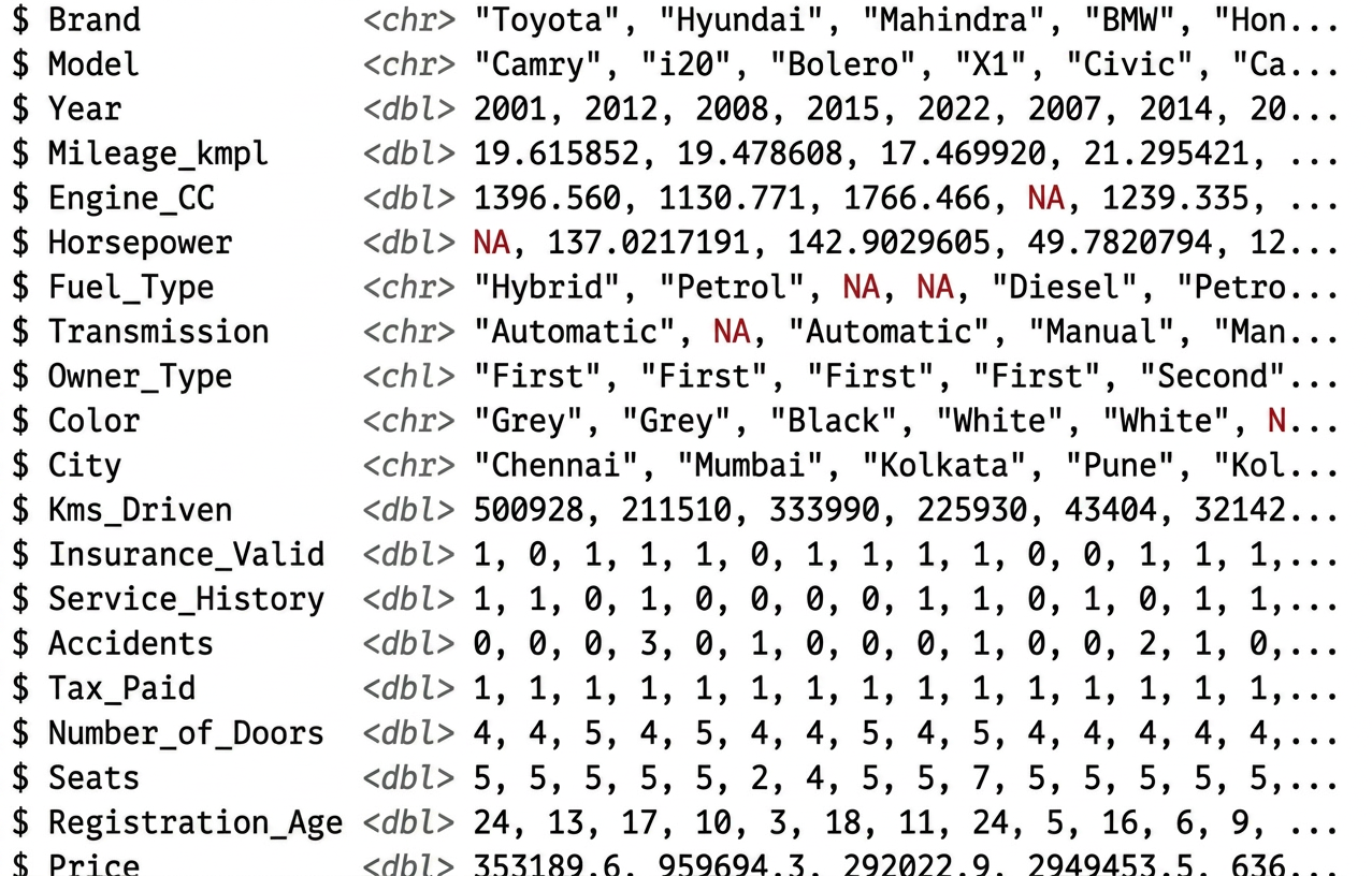
Missing Summary
missing_summary <- df %>% summarise(across(everything(), ~ sum(is.na(.)))) %>% pivot_longer(everything(), names_to = "Variable", values_to = "Missing_Count") %>% mutate( Total_Rows = nrow(df), Missing_Percentage = (Missing_Count / Total_Rows) * 100 ) %>% arrange(desc(Missing_Count))## Plot ggplotmissing_summary %>% filter(Missing_Percentage > 0) %>% ggplot(aes(x = reorder(Variable, Missing_Percentage), y = Missing_Percentage)) + geom_bar(stat = "identity", fill = "indianred", width = 0.7) + geom_text(aes(label = sprintf("%.1f%%", Missing_Percentage)), hjust = -0.2, size = 3.5, color = "black") + coord_flip() + scale_y_continuous(limits = c(0, 10)) + labs( title = "Variables with Missing Values", subtitle = "Showing only columns with missing percentage > 0%", x = "Variables", y = "Percentage of Missing (%)" ) + theme_minimal()
เราใช้ sumarise ในการวิเคราะห์ stat เบื้องต้นได้ว่าข้อมุลเราเป็นยังไง จาก code นี้เราใช้สำหรับการหา missing value หรือ NA ทุก column ด้วย across everything แล้วทำการ sum NA ให้หมดทุก Column และนี่คือผลลัพธ์ที่ได้
Missing summary
| Variable | Missing_Count | Total_Rows | Missing_Percentage |
| City | 80430 | 1005000 | 8.0% |
| Color | 80419 | 1005000 | 8.0% |
| Engine_CC | 80403 | 1005000 | 8.0% |
| Horsepower | 80403 | 1005000 | 8.0% |
| Mileage_kmpl | 80390 | 1005000 | 8.0% |
| Transmission | 80385 | 1005000 | 8.0% |
| Fuel_Type | 78733 | 1005000 | 7.83% |
| Brand | 0 | 1005000 | 0 |
| Model | 0 | 1005000 | 0 |
| Year | 0 | 1005000 | 0 |
| Owner_Type | 0 | 1005000 | 0 |
| Kms_Driven | 0 | 1005000 | 0 |
| Insurance_Valid | 0 | 1005000 | 0 |
| Service_History | 0 | 1005000 | 0 |
| Accidents | 0 | 1005000 | 0 |
| Tax_Paid | 0 | 1005000 | 0 |
| Number_of_Doors | 0 | 1005000 | 0 |
| Seats | 0 | 1005000 | 0 |
| Registration_Age | 0 | 1005000 | 0 |
| Price | 0 | 1005000 | 0 |
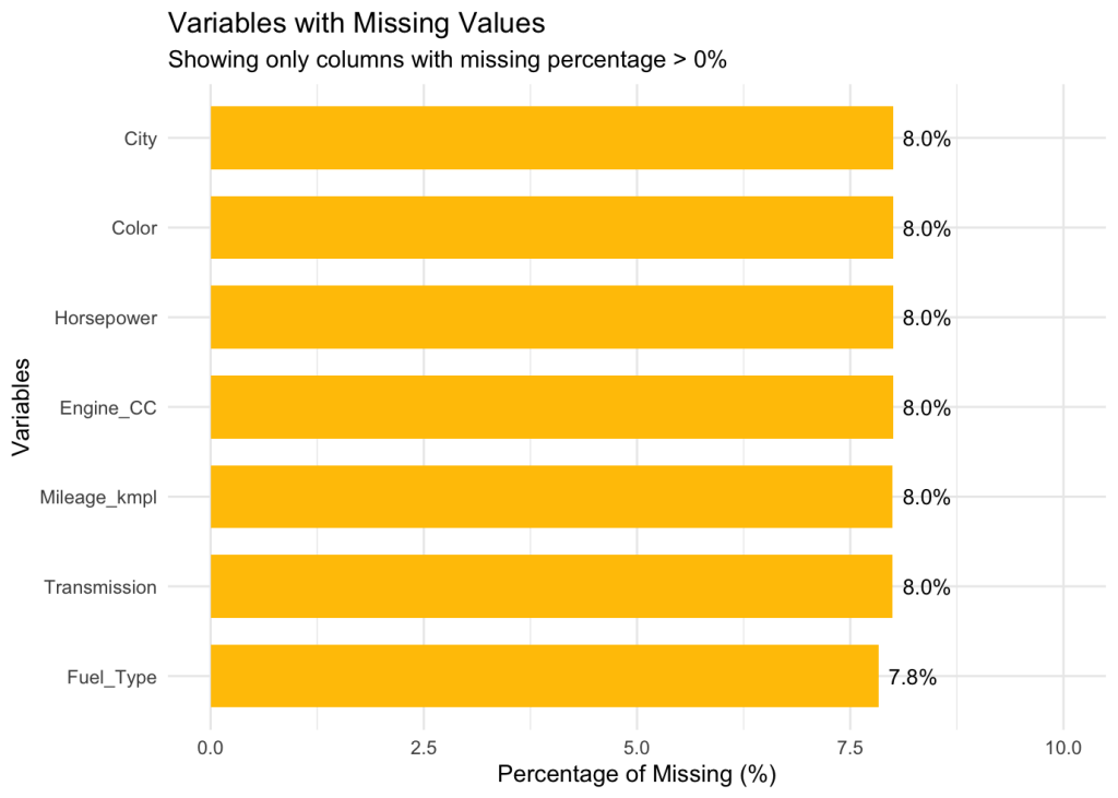
ggplot อ่านได้ที่ Reorder a variable with ggplot2
Key Findings:
- 1,000,000 + Rows
- 20 feature
- missing value ~ 8 %
Typo and Duplication
ถ้าข้อมูลไม่เยอะ ดูด้วยสายตาพาไล่มองเห็น สามารถใช้ unique มาช่วยได้กลั่นข้อมูลที่ซ้ำๆกันออกมาในแต่ละ feature
# Finding Typo & correlation year / refrigeration_agevvlapply(df %>% select(where(is.character)), unique)correlation_value <- cor(df$Year, df$Registration_Age)
หรือ เราสามารถหาได้จากการสร้าง control flow ขึ้นมาให้วิ่งไปดูการกระจายตัวของข้อมูล ทั้ง numeric และ character หากข้อมูลเยอะมาก
# Summary Statistics for Numeric Variablesnumeric_cols <- df %>% select(where(is.numeric))print(summary(numeric_cols))# Category Counts for Key Categorical Variablescat_cols <- df %>% select(where(is.character)) %>% colnames()for (col in cat_cols) { print(paste0("Distribution for:", col)) print(df %>% count(!!sym(col), sort = TRUE) %>% head(10))}
Key finding :
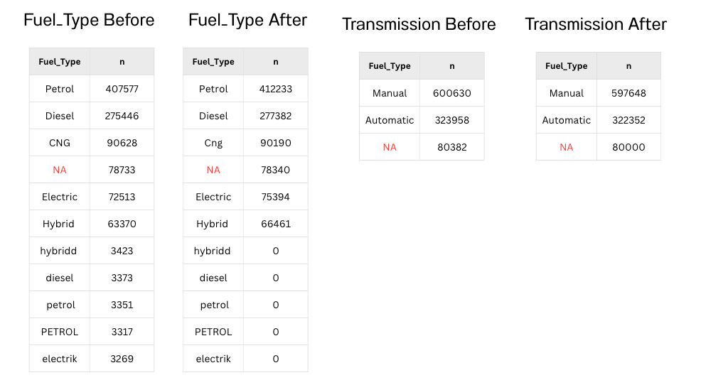
- I found some data inconsistencies in the Fuel_Type field. There are spelling and capitalization errors like diesel/Diesel, Electric/electrik, Hybrid/hybridd, and petrol/Petrol that we need to clean up.
- Yaer & Registration_age มี correlation กันที่ -1 ดังนั้นเราสามารถเลือกใช้ตัวใดตัวหนึ่งได้
- Missing values: Horsepower, Fuel_Type, Transmission, Color, City, and Mileage_kmpl have missing values. Consider imputation.
- numeric imputatuin with median group
- Character imputation with mode
- Skewed target: Price is highly skewed. A log-transform (log10 or ln) might improve regression modeling performance.
Data Cleaning
- drop duplicate
# Duplicatebefore <- nrow(df)# drop_duplicatesdf <- df %>% distinct()# check how many row dropremoved_rows <- before - nrow(df)
ก่อนหน้ามีที่หมด 1,005,000 row และเมื่อเราทำการลบค่าว่างออกไปด้วย distinct() แล้ว จะเห็นว่า removed_rows มีทั้งหมด 5,000 raw
- Fix Typos in Categorical Columns
ก่อนที่เราจะทำการ fix ค่าที่เขียนผิด หรือคำที่ต่างจาก group อื่นๆ แนะนำว่าอย่าลืม backup files ไว้เสมอ ห้ามเขียนทับไฟล์ต้นฉบับเด็ดขาด ! เผือว่าเราอาจจะเผลอไปลบค่าจริง จะทำให้ไม่สามารถย้อนกลับได้ หรืออาจจะต้องเสียเวลาในการ query data ใหม่อีกรอบ
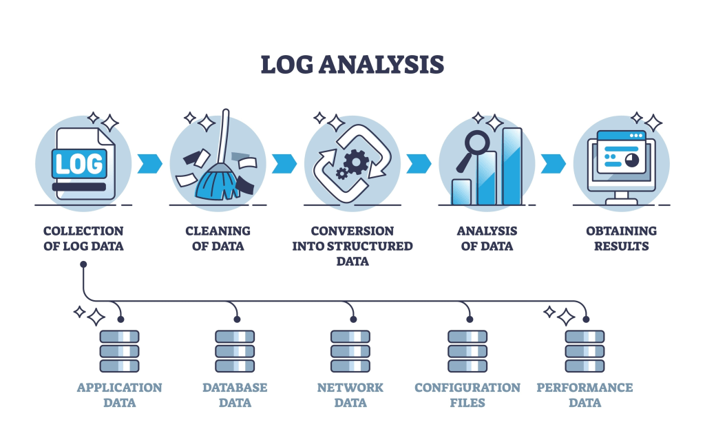
เรามาเร่ิมการ fix typo ของ Fuel_type กันเลยด้วยการ map ค่าที่ถูกต้องไปที่คำที่ไม่ถูก
# Fix Typo on Column Fuel_type# Named Vectorfuel_map <- c( 'petrol' = 'Petrol', 'PETROL' = 'Petrol', 'diesel' = 'Diesel', ' Diesel' = 'Diesel', 'DIESEL' = 'Diesel', 'electric' = 'Electric', 'electrik' = 'Electric', 'ELECTRIC' = 'Electric', 'hybrid' = 'Hybrid', 'hybridd' = 'Hybrid', 'HYBRID' = 'Hybrid', 'cng' = 'CNG')
ก่อนจะเอาไปแมพ เราจะทำการ str_trim() ก่อน หรือก็คือการลบ white space ที่ติดมา เพราะไม่รู้รู้ว่าไฟล์ที่โหลดมามี white space ไหม เพื่อความคลีนของข้อมูลก่อนนที่เราจะ map นั่นเอง
# ลบช่องว่าง -> เปลี่ยนคำตาม Map -> เปลี่ยนเป็น Title Case (ยกเว้น CNG)df <- df %>% mutate( # delete white space Fuel_Type = str_trim(Fuel_Type), # compared Fuel_type = fuel_map Fuel_Type = recode(Fuel_Type, !!!fuel_map), # chang title case Fuel_Type = str_to_title(Fuel_Type) )
** กฎเหล็ก: การทำ Data Cleaning ที่ดีคือการทำให้กระบวนการสามารถตรวจสอบย้อนกลับ (Reproducible) ได้เสมอ !
ทำการเปลี่ยนในทุก colomn เป็นรูปแบบเดียวกันทั้งหมด
# target_cols เปลี่ยนให้เป็นรูปแบบเดียวกันทั้งหมดtarget_cols <- c('Transmission', 'Owner_Type', 'Color', 'City', 'Brand', 'Model')df <- df %>% # Composition of functions (lambda fuction) mutate(across(all_of(target_cols), ~ str_to_title(str_trim(.x))))cat("Fuel_Type after cleaning:\n")df %>% count(Fuel_Type, sort = TRUE) %>% print()cat("\nTransmission after cleaning:\n")df %>% count(Transmission, sort = TRUE) %>% print()
- missing value (pt 101)
- numeric imputatuin with median group
- create factors med_cols
- control flow (for)
- numeric so easy ! 🍌
- numeric imputatuin with median group
# Missing Value managements# median med_cols <- c('Mileage_kmpl', 'Engine_CC', 'Horsepower')for (med_col in med_cols) { # calculate median median_val <- median(df[[med_col]], na.rm = TRUE) # replace NA with Median df[[med_col]][is.na(df[[med_col]])] <- median_val # result cat(sprintf(" '%s' → filled with median = %.2f\n", col, median_val))}
- missing value (pt 102)
- Character imputation with mode
- create factors
- calculate NA with tabulate() = สำหรับนับควสมถี่ คล้ายผล vote จากการ match(x, ux)
- control flow (for)
- Character imputation with mode
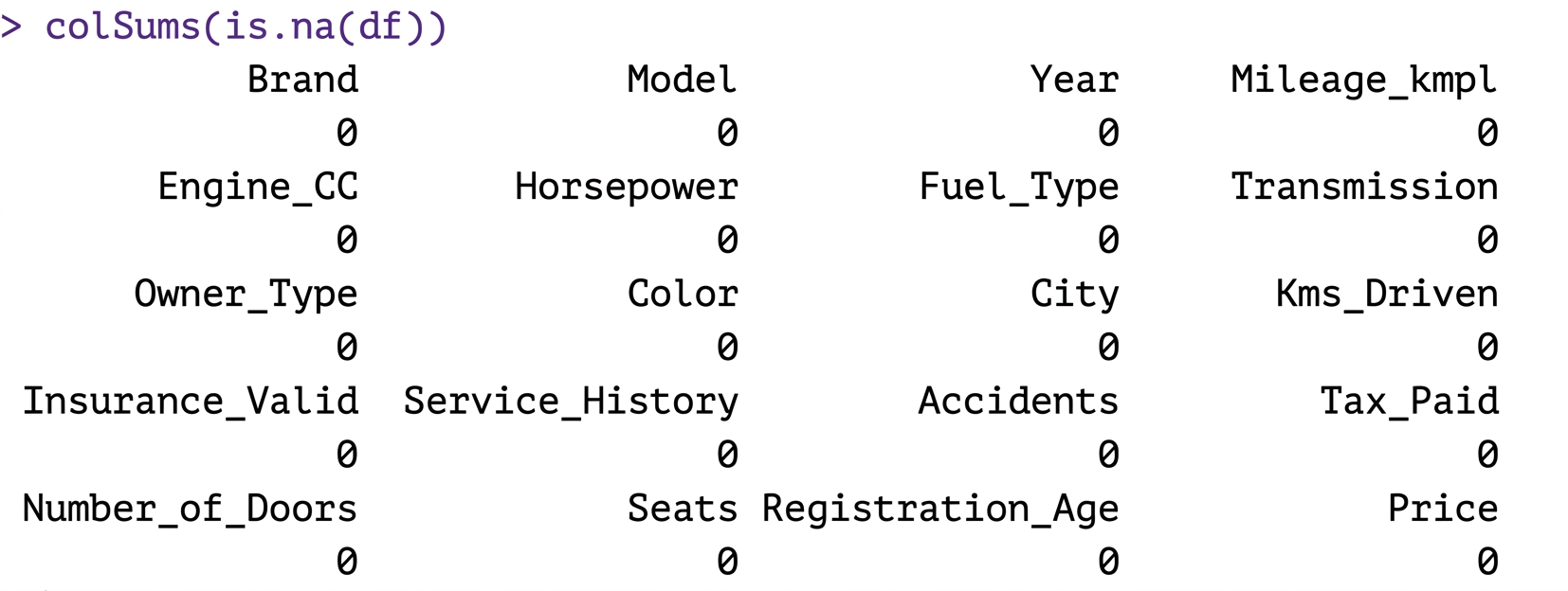
# Missing Value managements# modemod_cols <- c('Fuel_Type', 'Transmission', 'Color', 'City00')get_mode <- function(x) { x <- x[!is.na(x)] # ตัดค่า NA ทิ้งไปก่อนคำนวณ if (length(x) == 0) return(NA_character_) #ถ้าไม่มีข้อมูลเ00ย ให้คืนค่า NA ux <- unique(x) #หาคำที่ไม่ซ้ำกันในคอลัมน์ #นับจำนวนคำ และดึงคำที่ซ้ำบ่อยสุดออกมา ux[which.max(tabulate(match(x, ux)))]} for (mod_col in mod_cols) { # หาคำซ้ำ mode_val <- get_mode(df[[mod_col]]) # แทนที่ค่า NA ในคอลัมน์นั้นๆ ด้วยค่า Mode (ฐานนิยม) df[[mod_col]][is.na(df[[mod_col]])] <- mode_val cat(sprintf(" '%s' → filled with mode = %s\n", mod_col, mode_val))}
*** อธิบาย mode ง่ายๆ : ตัวเลข (match) -> นับคะแนนใส่ถัง (tabulate) -> หาเบอร์ที่ชนะโหวต (which.max) -> แล้วหงายหน้าเปิดดูว่าเบอร์นั้นคือคำศัพท์คำว่าอะไร (ux[...]) และตอนนี้เมื่อเราเช็ค NA ก็จะเห็นว่าไม่มีแล้ว เย้ !
- Outlier Removal (IQR × 3)
target_cols <- c('Price', 'Kms_Driven', 'Engine_CC', 'Horsepower', 'Mileage_kmpl')# สั่งกรองข้อมูลรวดเดียวจบด้วย if_alldf_clean <- df %>% # 1. กรองปีให้อยู่ในช่วง 1995 - 2025 filter(Year >= 1995 & Year <= 2025) %>% # 2. กรอง Outlier โดยใช้ if_all filter(if_all(all_of(target_cols), ~ { q1 <- quantile(.x, 0.25, na.rm = TRUE) q3 <- quantile(.x, 0.75, na.rm = TRUE) iqr_val <- q3 - q1 # return TRUE/FALSE กลับไปให้ filter เลือกเก็บเฉพาะแถวที่ผ่าน .x >= (q1 - 3 * iqr_val) & .x <= (q3 + 3 * iqr_val) }))# สรุปจำนวนแถวและคอลัมน์สุดท้ายcat(sprintf("\n Final clean dataset: %s rows × %d columns\n", format(nrow(df_clean), big.mark=","), ncol(df_clean)))
Final clean dataset: 990,840 rows × 20 columns
What’s Next Pt102? 🎧
Exploratory Data Analysis
- A. Price Distribution (Target Variable)
- B. Relationships: Numeric Variables vs. Price (Sampled for speed due to 1M rows)
- C. Categorical Variables vs. Price (Boxplots)
- D. Correlation Matrix of Numeric Variables


Leave a comment